Introduction
Here we walk though the most basic approach to using MEOW-HiSS to simulate the arrival and profile of a HSS at 1 AU. The full OSPREI distribution is not needed for this, only two files that are included within it. We require empHSS.py from the coreCode folder and predMEOWHiSS.py from the processCode folder. If you scroll to the bottom of predMEOWHiSS.py you will see several examples of how to call predfromCH (comment out), which is the main function to convert from measured coronal hole (CH) parameters to the expect 1 AU profiles. For example:
predfromCH(34, gridscale=True, userAmb=[8, 330, 2.5, 3.5, 50000], t0='2016/09/16 13:30', omniname='omniSep2016.dat', plotstart='2016/09/18 13:30', plotstop='2016/09/23 18:30', obsstart='2016/09/19 04:00', obsstop='2016/09/22 22:00', savename='MHpred_Sep16.png')
was used to generate the September 2016 example from the MEOW-HiSS paper. We cannot yet run MEOW-HiSS with all these details, so to start try simply
predfromCH(34, gridscale=True) You can either just add this line at the bottom of predMEOWHiSS.py or import predMEOWHiSS into a python environment and call it there. However you run it, the figure shown to the left should pop up. The dashed blue line shows the expected number density, radial velocity, radial magnetic field, longitudinal magnetic field, temperature, and longitudinal velocity. Note that the absolute values of the magnetic field and longitudinal velocity are shown. Right now, the only parameter we have provided is the size of the CH used to generate the HSS. This is the "34" in the call and we have set the optional parameter "gridscale" to True that this means 34 grid units. Alternatively, if gridscale is set to False then the CH area should be given in 108 km2. The default is False if gridscale is not specified. Since we have not set an actual time, the x-axis is showing time relative to the first time that our theoretical CH contacted the Sun-Earth line. The different colored regions correspond to the stream interaction region (SIR, leftmost 3 regions), the plateau, and the tail. The rest of the demo will walk through the different parameters and how to set them. Note that useful times are printed to the command line. First and final contact are fairly self-explanatory and the HSS front uses the traditional definition of where the longitudinal flows reverse direction, which is at the front of the last region in the SIR.
Coronal Hole Parameters
As we've seen MEOW-HiSS really only needs the CH area and timing of first contact with the Sun-Earth line to generate full in situ profiles. The easiest way of getting these values is to just use JHelioviewer, though we cannot guarantee this method will always work to do actual "predictions" depending on the availability of near-real time data. One could easily craft their own method using a source with real time availability, but we have not done this.
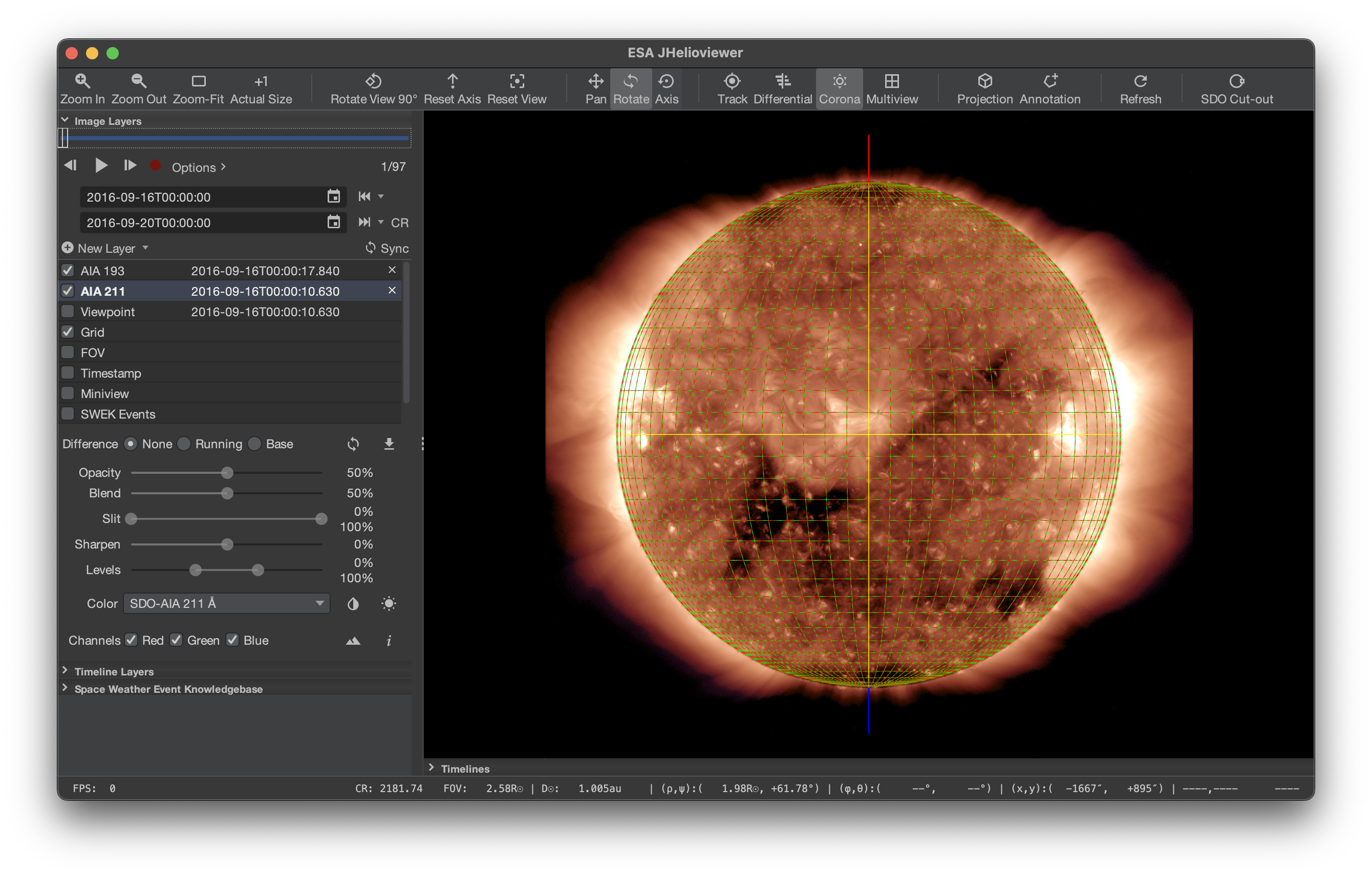
Download and install JHelioviewer on your system if you do not already have it. Open it and set the time range from 2016-9-16T00:00 to 2016-09-20T00. Next add a layer with SDO AIA 193, followed by a layer of 211. It will probably take some time to load the data. 193 should be on top of 211 in the layer list and set the opacity of 211 to 50%. It looks best this way even though CK does not know why having something at 50% opacity below something at 100% opacity is visible at all (try toggling the layers on and off and switching their order). CK also turns off the Miniview and SWEK Events to make the screen less cluttered then zooms in on the image panel. The CH we are interested in should be in the bottom left quadrant of the image.
Click on Grid so that the grid settings come up in the bottom of the left panel. Change both the longitude and latitude resolution to 5 deg and unselect Grid labels if you want to remove the excessive amount of labels we have created. Everything is now configured to start finding our CH inputs. The following figure shows the settings after configuration.
Start advancing in time until the CH reaches the central meridian. Defining this exact time is a bit of an art form. CK suggest looking for the first contact of a bulky part (as opposed to a fine scale extention) and preferably something closer to the equator as opposed to toward the poles. For this paper version of this case, CK decided it was somewhere between 13:00 and 14:00 on 16 Sep and used 13:30. If you add "t0='2016/09/16 13:30'" into the call to predfromCH you should get the same results, but with a real time x-axis.
Next, we just have to count the number of grid cells that the CH covers. Move the time forward so that the CH is as Earth-directed as possible (centered around the meridian), which should minimize any projection effects. For the paper, CK used a time of 05:02 on 17 Sep. Panel a of the figure below shows this time. CK also has no clue why her JHelioviewer times are now a few minutes different from what was done previously and suspects it may be related to which source is used for the SDO images, but this difference of a few minutes does not really matter. Count the number of grid cells which contain any bit of CH. MEOW-HiSS tends to perform better with larger CH sizes so be generous on including cells. Panel b uses a blue outline to show the region that was considered CH. This is a total of 34 grid cells, which is what we pass to MEOW-HiSS for the CH area.

As mentioned, this is may not an option that works for real time predictions. At the time of writing this demo (Feb 2024), JHelioviewer did contain SDO images from within the last hour but there is no guarantee of this level of availability in general. It would not be complicated to project a grid onto a different source of real time images and perform a similar analysis or even use a more sophisticated image processing technique to extract the dark CH area.
Observations
The next option is to include actual observations for comparison to the MEOW-HiSS results. The OMNI database is an easy way of doing this. We want to pass it a file with the format year, DoY, hr, Bx, By, Bz, T, n, v, flow lon, flow lat. The lower resolution, hourly data is available here. Switch the webform from Plot data to List data and enter start and stop days as a few days or a week before and after when you expect the HSS to pass over the Earth. Deselect IMF Magnitude Avg but select Bx, By, Bz (in GSE), Proton Temperature, Proton Density (probably already selected), Flow Speed, Flow Longitude, and Flow Latitude. Hit submit and a list should appear. Copy and paste the data (you can skip the header) into a text file. Alternatively, you can pull this information via the command line
curl -d "activity=retrieve&res=hour&spacecraft=omni2&start_date=20160914&end_date=20160930&vars=12&vars=13&vars=14&vars=22&vars=23&vars=24&vars=25&vars=26" https://omniweb.gsfc.nasa.gov/cgi/nx1.cgi > omniSep2016.dat  Note that some terminals have strong feelings about copying and pasting quotation marks from different sources so if you get an error you might want to try replacing them with directly-typed versions. Open up the output file and remove the header and footer information. You can now pass this file to the MEOW-HiSS command using "omniname='omniSep2016.dat'" and the figure will include the observed data. We do check Bx for bad data, if you run into cases with other bad data you may need to add to the code or just manually remove it. For this case we get a pretty good agreement on the arrival time of the HSS and the general profiles. The longitudinal velocity comparison isn't great. This is a known issue and MEOW-HiSS does seem to accurately reproduce the MHD simulations it is based on, but these don't particularly match the observed lateral flows. This isn't the most critical of parameters so improving it is not a current priority.
Tuning SW Parameters
MEOW-HiSS is designed to add a HSS on top of a quiescent background solar wind model. The values it returns are coefficients by which to multiply the steady state values, except for the longitudinal velocity since a basic SW model would set this to zero. preMEOWHiSS is set up to run using default values for the solar wind parameters at 1 AU (7.5 cm-3 for the density, 350 km/s for the velocity, 4.2 nT for both Br and Blon, and 75000 K for T). You can adjust these parameters to better match the observed upstream, ambient solar wind if you have estimates of those values. Add userAmb=[8, 330, 2.5, 3.5, 50000] into the function call. Running the program now produces the same dashed blue line using the default ambient values and a red line using the tuned SW parameters. These estimated values are not all that different from the default SW values, the most noticeable change is in Br, and the improvement in the ambient values leads to a slight improvement in the magnitude of the peak in the profile. If you wish to turn off the default blue line you can add "plotdefAmb=False" to the call.
Tuning Image Parameters
The remaining options are all just fine tuning the image aesthetics. The optional parameters plotstart and plotstop set the boundaries of the image (e.g. plotstart='2016/09/18 13:30' within the call). If the observed HSS boundaries are known then they can be included via optional parameters obsstart and obsend (e.g. obsstart='2016/09/19 04:00'). This will add vertical lines at these times within the plot. It also will calculate the mean error in each parameter, both in physical units and weighted by the ambient value to get a percentage error. These values are printed to the terminal. Finally, one can specify a name to save the figure instead of just displaying it by setting the optional parameter savename (e.g. savename='MHpred_Sep16.png').
- © CK 2023
- Design: HTML5 UP