2. Basic interplanetary OSPREI
2.1 Running your first test case
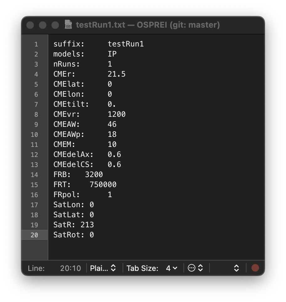
We’ll start by running the testRun1.txt case from the exampleFiles folder. This a minimal example of an IP run to check that everything is working and get used to the procedure. Either run
python OSPREI.py exampleFiles/testRun1.txt
or move the .txt file to the top directory and run
python OSPREI.py testRun1.txt
A series of numbers will go by. On a brand new 2023 Macbook Pro it takes a couple seconds. On an older computer it may take closer to a minute. The first few lines will look like:
   0.02  21.60 1198.73  46.00  18.00   0.60   0.60 11653.18   5.87 5300.31   0.00   0.00   0.00
  0.17  22.52 1188.03  46.00  18.00   0.59   0.59 10318.56   5.86 5015.49   0.00   0.00   0.00
  0.33  23.54 1177.52  46.01  18.01   0.59   0.58 9068.72   5.84 4722.10   0.00   0.00   0.00
  0.50  24.54 1168.17  46.02  18.03   0.58   0.57 8013.52   5.82 4449.52   0.00   0.00   0.00
  0.67  25.54 1159.71  46.04  18.07   0.57   0.56 7114.24   5.80 4195.21   0.00   0.00   0.00
This shows the simulation time (hr), CME front distance (Rs), CME radial (speed), face on AW (°), edge on AW⊥ (°), aspect ratio of the axis (δAx), aspect ratio of the cross section (δCS), CME number density (cm-3), log(temperature) (K), magnetic field parameter B0 (nT, field at axis is δAxB0), yaw (°), rotational speed (°/hr), and region number useful for HSS cases. Note both AW are technically half widths, which is the commonly used definition in the field.
These will continue printing at set intervals until the CME reaches the satellite. Upon first contact, a second line begins printing below the first line and slightly indented:
 56.60 213.53 470.33  55.03  28.14   0.30   0.26   5.66   4.78  93.69   0.00   0.00   0.00
       sat1  0.98004  0.00057 -0.00005
 56.70 213.77 470.09  55.04  28.15   0.29   0.26   5.64   4.78  93.56   0.00   0.00   0.00
       sat1  0.97092  0.00057 -0.00005
 56.80 214.01 469.85  55.04  28.16   0.29   0.26   5.62   4.78  93.44   0.00   0.00   0.00
       sat1  0.96182  0.00057 -0.00005
 56.90 214.25 469.61  55.05  28.17   0.29   0.26   5.59   4.78  93.31   0.00   0.00   0.00
       sat1  0.95274  0.00057 -0.00005
This lists the satellite name (default of sat1, more on multiple satellites later) and the location of the satellite within the CME at that time. We show the fractional radial distance, the toroidal angle (0° nose, ±180° flanks), and the poloidal angle (0° front/entering, ±180° rear/exiting). This is a useful way of tracking where the satellite is if any results are looking weird or difficult to interpret.
Finally, at the bottom, it should print out:
Satellite:         sat1
Transit Time:      56.38333333333333
Final Velocity:    470.85985715489454 35.341976415963885
CME nose dist:     213.0037845064749
Sat. longitude:    0.0
Est. Duration:     26.31666666666667

0 Contact after 2.36 days with front velocity 470.86 km/s (expansion velocity 35.34 km/s) when nose reaches 213.53 Rsun and angular width 55 deg and estimated duration 26 hr
   Density:  5.658109547769871   Temp:   60190.49915787337
You should have an exact match to these values. This lists several useful results for this simulation. A lot of information is repeated, but the top half (list) comes from ANTEATR when it is not running in silent mode and the bottom half (sentence) is from OSPREI. The “0” in front of the sentence is an ID number, not “zero contact.” When running an ensemble this will start at 0 for the seed case and count upward for each member.
If you look in your top directory a new folder named NoDate should have appeared. OSPREI likes to keep things organized rather than dumping all the outputs into the main folder. If you are running a case with an actual date then it will create a folder for that date (e.g. 20120712 for the 2012 July 12 CME). In this case, we are looking at a generic CME so it created a NoDate folder. All generic results will live in this folder.
Open NoDate and inside there should be two files (ANTEATRresultstestRun1.dat and FIDOresultstestRun1.dat) that contain the results of our simulation. The full description of each column within these files is given in the appendix.
2.2 Visualizing your first results
OSPREI comes with processing scripts that take the standardized result files and generate whatever figures are relevant for the current configuration. Run:
python processOSPREI.py IPexMin.txtand three new figures (fig_testRun1_DragLess.png, fig_testRun1_IS.png, fig_testRun1_Jmap.png) should appear in NoDate. Nothing important is printed to the command line for this case, the few lines that appear are just the OSPREI check for which components are running and whether it is doing an ensemble.
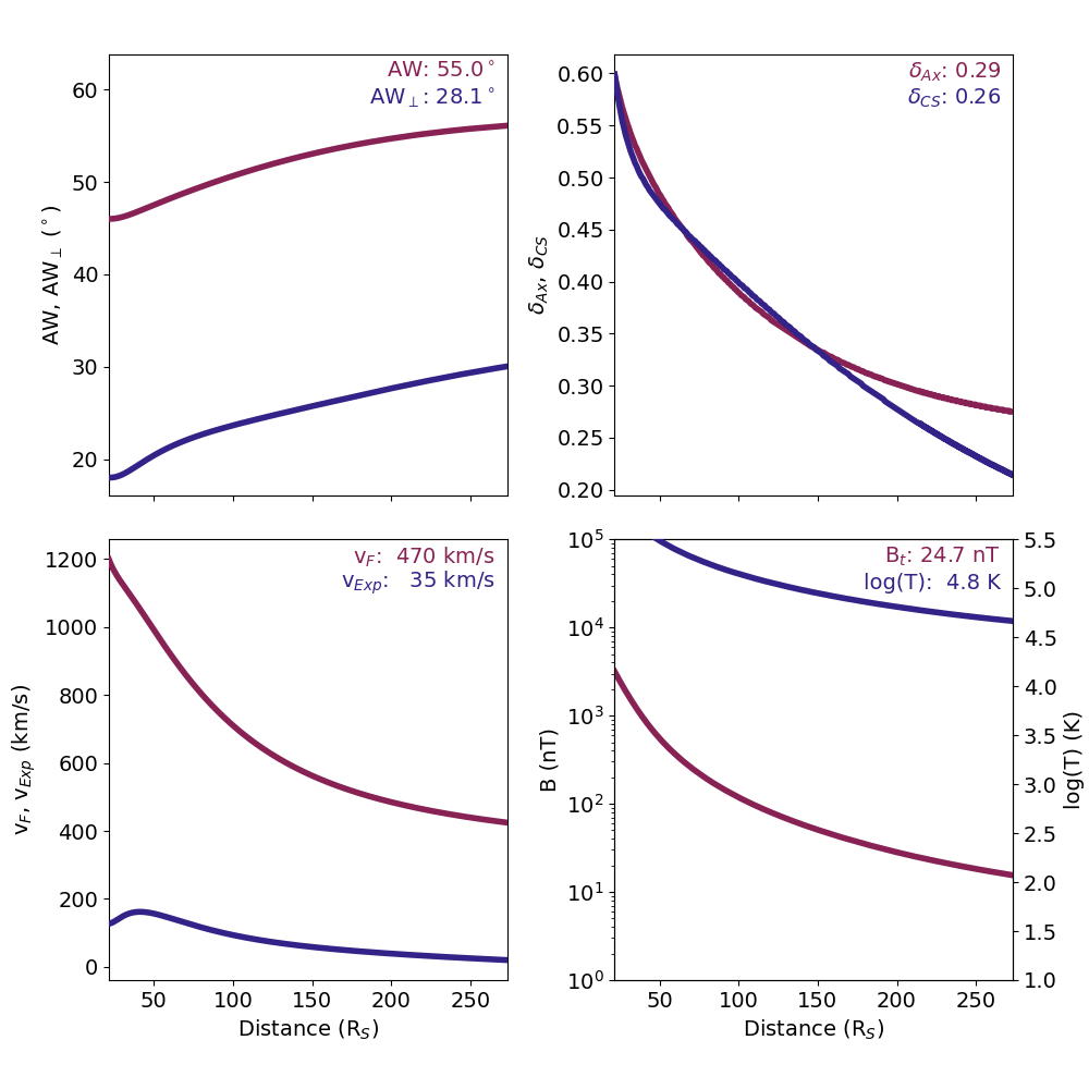 The DragLess figure shows the evolution of a limited number of parameters from the OSPREI simulation. This figure is meant to be easy to interpret quickly but contain the essential properties for potential forecasts. The top left shows the expansion via the evolution of AW (maroon) and AW⊥ (blue). The top right shows deformation via the aspect ratios δAx (maroon) and δCS (blue). The bottom left shows the propagation via vr (maroon) and vexp (blue). The bottom right shows the evolution of the internal B (maroon) and log(T) (blue). The numbers in the top corner of each panel show the values when the flux rope makes first contact with the satellite. This figure is entirely automated and tries to get the best range for each panel, but there will sometimes be overlap with the text. This is fine if one is trying to just get a sense of the behavior but the plotting script may need to be tuned for publication quality figures.
 The J Map figure is similar to the J maps produced from observations, but subtlely different since it is derived from model results. At each time, we determine the width of the CME along the radial path connecting the center of the Sun and the satellite of interest. This region is then just stacked in the horizontal direction, showing the evolution of the width and distance over time. If we included a CME-driven sheath then the figure would show two regions with a maroon region showing the sheath upstream of the gray CME region. The horizontal dashed line represents the distance of the satellite, in this case our near-Earth satellite at L1.
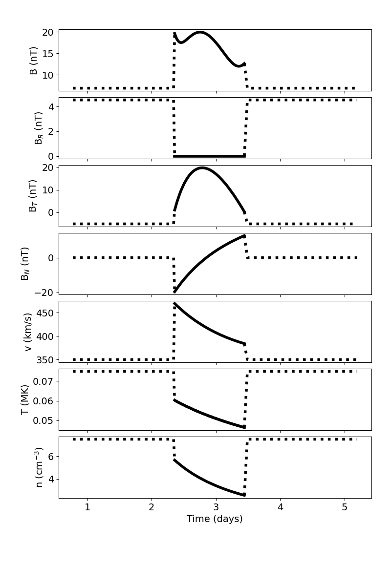 The IS figure shows the in situ profile that would be observed for this case. From top to bottom it shows the total magnetic field (B), the vector components, the radial velocity, the temperature, and the number density. FIDO defaults to showing the magnetic field in satellite coordinates (RTN). It can be switched to an "Earth-mode" by setting isSat to False in the input file. In Earth-mode, the magnetic field will be shown in GSE coordinates and the number density is replaced by an estimate of the expected Kp index. Within each panel, the solid region corresponds to the flux rope signature and the the dotted region is the solar wind surrounding the CME. If we included a CME-driven sheath it would appear as a dashed line ahead of (to the left of) the flux rope portion. For a generic simulation such as this (opposed to one with a given date) the x-axis appears as days from the start of the simulation.
2.3 Understanding inputs
The input file controls all of the OSPREI parameters. Open IPexMin.txt with a text editor and we will go through the options used in this first example. The file has two columns, the first is a list of inputs and the second is the corresponding values. The input names must exactly match one of the keywords that OSPREI expects and have the “:” at the end to be recognized. The Appendix includes a list of all possible input parameters.
 In our test case, suffix is the first parameter, which we have set to "demo." This gives OSPREI a name to tag all the simulation results with, which is why all our data files and figures included demo in their name. This allows you to perform multiple simulations that will live in a single date/NoDate folder without overwriting one another as long as they have different suffixes.
The second input is which models to run, which we have set to "IP". This can be any of [All, IP, noB, FCAT, ANT, FIDO], where noB is ForeCAT and ANTEATR without any in situ profiles. We then set nRuns to the number of cases to run. For now we keep this at a single run, but this is where ensembles are set.
The next set of parameters that start with CME are the CME properties. This includes the position and orientation (radial distance in Rs, lat/lon/tilt all in degrees), the radial speed at the start of the simulation, the angular widths, the CME mass (in 1015 g), and the aspect ratios. Then we have flux rope (FR) parameters, which are the internal B (in nT) and T (in K) at the start of the simulation. FRpol sets the handedness of the flux rope with 1 being right handed (-1 for left handed). The orientation of the axial field is set by the sign of FRB.
The last set of parameters are the satellite (Sat) parameters with the position given in Rs and deg. SatRot sets the orbital speed of the satellite, which should be given in rad/s. Here we have set it to stationary, but if it is not explicitly provided it will default to the Earth’s orbital speed.
Try playing with the CME and FR parameters to get a sense of their effects. Start with small changes. If things get too crazy the simulation will quit when forces get unstable. In particular, ANTEATR depends on the magnetic forces of a curved flux rope and if the FR cross section gets too thick relative to how curved the axis is then the forces become unstable. If you swap AWp to 38 and run you can see it runs for a while then stops and says “ANTEATR-PARADE forces unstable.” If things are going wrong this is usually the thing to check first. Other errors can happen if FRB or FRT is too high so there is excessive expansion early on. Any (reasonable) coordinate system can be used for the CME/sat longitude when you are not using ForeCAT, just make sure you use the same one for both. Unexpected misses can occur if one longitude is in Stonyhurst while the other is in Carrington.
While exploring input parameters you may find that you had achieved the "perfect" simulation, but then kept changing things and forgot what the perfect parameters were. Don't worry, all of this has happened before and all of this will happen again, but there is an option that can help. As of SPD 2023, OSPREI includes the Enable Reproducibility with the Input Keeper Assistant (the ERIKA feature), which automatically logs the timestamp of each run and a complete record of the input parameters. This can be useful if you need to backtrack to figure out what worked better before. This information is stored in inputs.log in the same folder as the OSPREI outputs (either NoDate or the specific date). If you wish to turn this off then switch logInputs to False in the call to setupOSPREI near the bottom of OSPREI.py
Once you feel comfortable with this most basic form of OSPREI move on to the next section to see some of the more advanced options that are available.