5. Full OSPREI Runs
5.1 Running OSPREI
We can now run a full OSPREI run using the testRun5.txt input file (yes, we skipped 4). Pass this file to OSPREI and the full simulation should begin. If you changed anything in the naming schemes you might have an issue, but just make sure OSPREI points to the correct magnetic field folder. The pkl files are read in by ForceFields.py in the coreCode folder (lines 28 and 32) and they can be modified (if needed) to match your system and naming conventions.
Run OSPREI. The simulation now starts with:
Running ForeCAT simulation 1 of 1
  0.000   1.200 -29.000 350.000  60.000  50.000   0.000  10.619   0.802
  5.000   1.221 -28.994 349.981  60.130  50.000   1.954  11.157   0.923
 10.000   1.243 -28.975 349.928  60.469  50.000   3.601  11.684   1.050
which shows the progress of the ForeCAT simulation. These lines show the time (min), radial distance (Rs), latitude (°), longitude (°), tilt (°), radial speed (km/s), nonradial speed (km/s), AW (°), and AW⊥ (°).
OSPREI uses a three phase evolution for the CME’s radial velocity where it starts out slow then linearly accelerates until it reaches a constant value at the speed given. This constant speed is the only value that must be specified in the input file (CMEvr, the same as used to set the initial IP speed) but the initial speed (FCvrmin) and the distances of the transitions can also be specified (FCraccel1, FCraccel2) if you have estimates for them. If not provided, default values will be used. For this case we have set these values in the input file.
Similarly, the angular width initially expands as the CME begins rapidly accelerating. We use an exponential to take the CME from some small initial size to the final specified values. The AW is the only required parameter. AW⊥ will default to 1/3 of AW, which is somewhat arbitrary but reasonable, but it best to provide it if there is any educated guess. We tend to let the parameters controlling the the value of AW at 1 Rs (FCAWmin) and the length scale of increase (FCAWr) remain at the defaults.
ForeCAT will run until the CME reaches FCrmax, at which point ANTEATR starts, and the transition automatically happens with the code passing the necessary information between the components. In the input file we have turned on the CME-driven sheath but do not include a HSS or yaw rotation. The satellite is set directly within the input file, rather than passing a .sat(s) file, and the rotation is set static. These numbers are mimicking the location of Solar Orbiter for this event.
Back to our example case, OSPREI finishes with the following results:
0 Contact after 2.99 days with front velocity 335.40 km/s (expansion velocity 17.99 km/s) when nose reaches 127.02 Rsun and angular width 39 deg and estimated duration 20 hr
Impact at 2021 Sep 26 04:18
Density: 50.59647977035288 Temp: 19449.660034734094 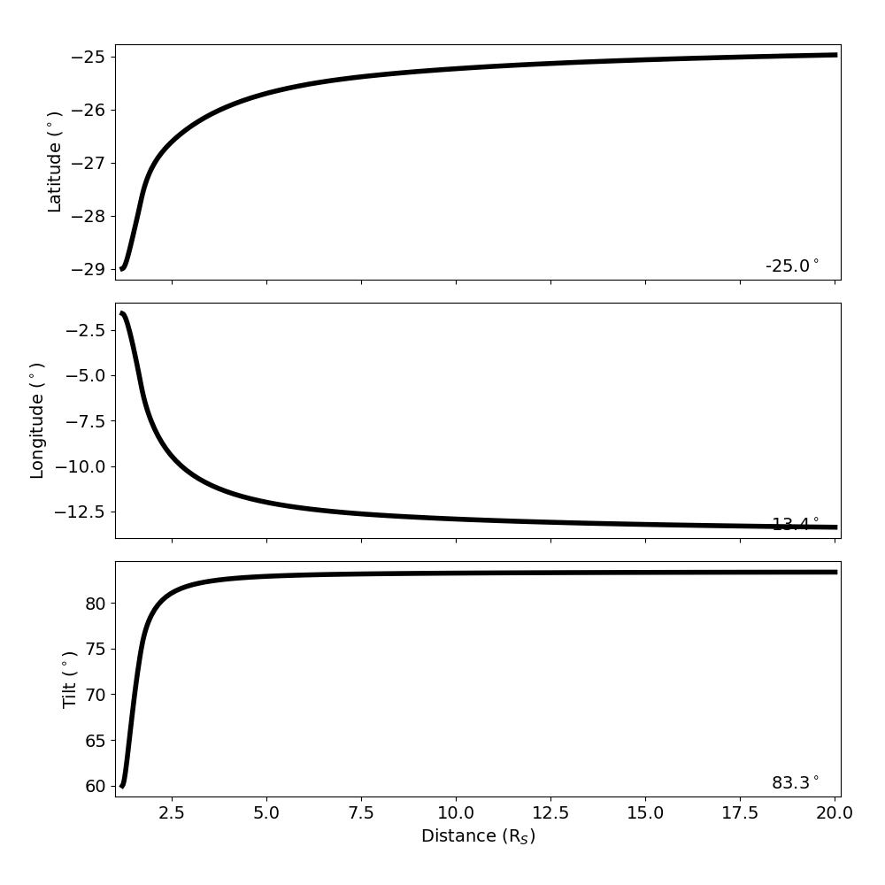 and a new results will appear in the 20210923 folder. It will contain all the IP results, as before, and a new ForeCAT results file.
5.2 Visualizations
Run processOSPREI.py and figures will be generated in the 20210923 folder. We get the same types of figures as before, plus a Central Position Angle (CPA) figure showing the deflection and rotation of the CME from ForeCAT. We see that this CME shows a few degrees of deflection in both latitude and longitude, as well as a few degrees of rotation.
This example corresponds to an observed CME so we have included the observed in situ data for this case. In the input file we set ObsDataFile to exampleFiles/20210923_soldata.dat, which has the format:
#Year DOY hour Btot Br Bt Bn Np Vtot Tp
2021 266 0 8.2 2.9 7.1 2.1 21 337.3 51124
2021 266 1 7.2 2.1 4.4 2.1 20 334.0 66889
2021 266 2 8.4 5.2 3.2 3.9 20 338.1 69730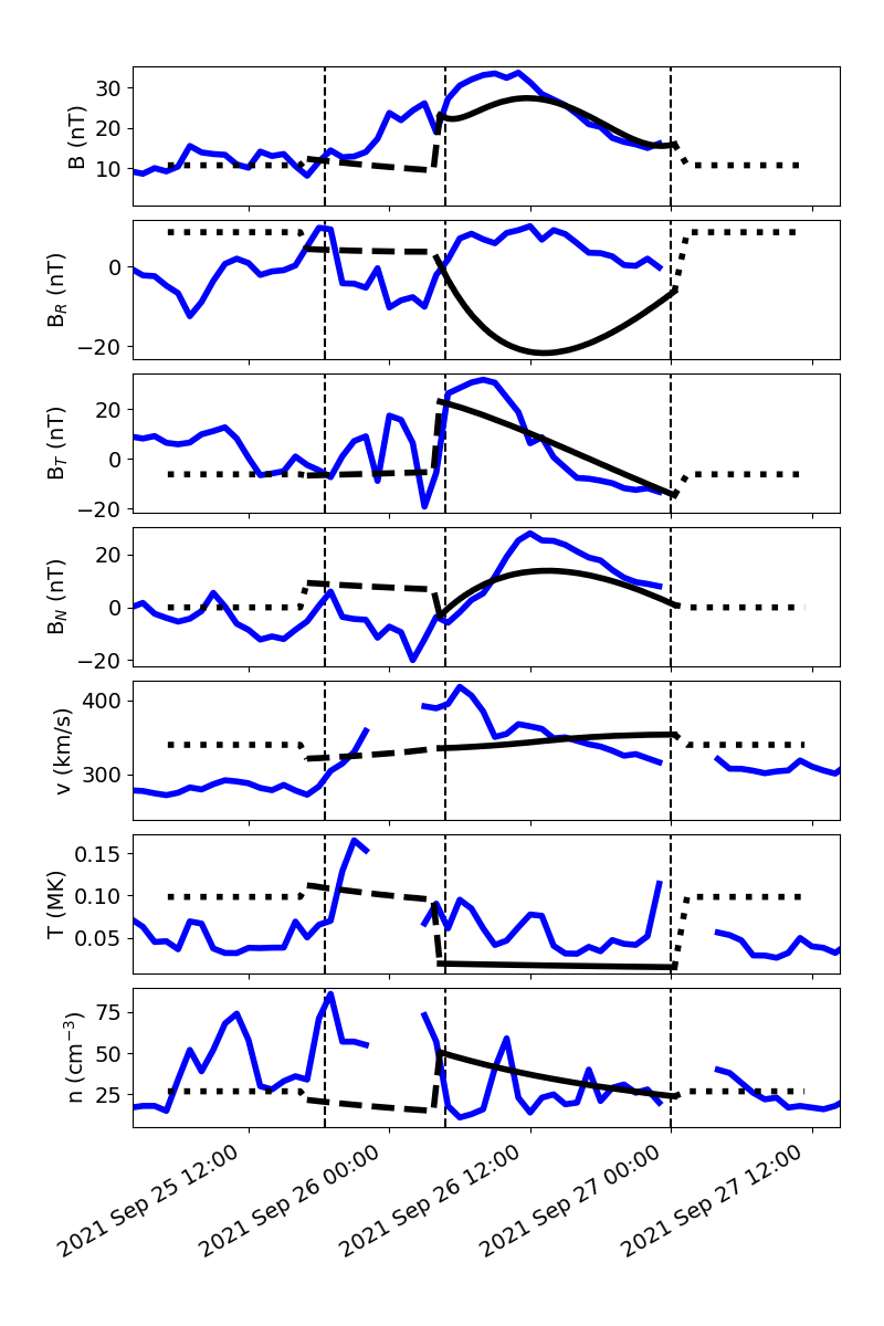 where the B values are in nT, number density in cm-3, velocity in km/s, and temperature in K. -9999 is used as a flag for missing/bad data. We have also given the observed sheath start and flux rope start and stop (obsShstart, obsFRstart, obsFRend) in the input file, all in fractional day of year. The in situ figure now makes use of all of this information. The black line shows the OSPREI results and the blue line the observed data. The vertical dashed lines show the observed boundaries. The dotted portion of the black line is the ambient SW. The amount of it included in front of and behind the CME can be adjusted using SWpadF and SWpadB (in hours) in the call to makeISplot in processOSPREI.py.
When running processOSPREI it will now return a set of scores that are calculated as a metric of comparison to the observational data. This output starts by listing which satellite the numbers are for (in this case, a generic “sat” because we have not provided a list of satellites with names). The lines of numbers are three sets of seven numbers. The three sets correspond to different time ranges, the full sheath+flux rope, just the sheath, and just the flux rope. If there is no observed sheath start given then it will just be one set of numbers for the flux rope. The seven numbers then correspond to the error in B/Bx/By/Bz/n/v/T.
----------------------- Sat:  -----------------------
0 4.779 17.092 8.936 9.178 20.691 27.955 39972.437   7.257 9.064 12.870 14.109 42.424 29.809 41006.710   3.474 21.317 6.866 6.583 13.828 27.370 39645.825


Average Errors (Full/Sheath/Flux Rope, B/Bx/By/Bz/n/v/T):
4.779 17.092 8.936 9.178 20.691 27.955 39972.437 7.257 9.064 12.870 14.109 42.424 29.809 41006.710 3.474 21.317 6.866 6.583 13.828 27.370 39645.825

Average Weighted Errors:
0.208 3.048 0.663 0.725 0.600 0.079 0.569 0.390 1.455 1.321 1.708 0.661 0.086 0.364 0.137 4.038 0.445 0.440 0.551 0.077 0.698

Seed has total score of  5.988808429990655
Best total score of  5.988808429990655 for ensemble member  0
The first line lists the OSPREI run number (0 in this case because it is a single run), then the mean absolute error for each parameter over each range (in nT, cm-3, km/s, and K). If we ran an ensemble we would see one line for each member. The line labeled average errors is then the average of each value over all ensemble members. As we did a single run, this is the same as the single member line. The weighted errors normalize each value by the average observed value of that parameter over the appropriate duration, giving a unitless, fractional error.
We combine these errors with a measure of the timing accuracy to determine a single number quantifying the quality of fit to the observations. The timing error is calculated around line 2749 (timingErr). We calculate a timing error equal to the absolute error in days for each of the observed boundaries. The combined error is determined around lines 160-172 in proMetrics.py. Farther down, around line 314 want2use options list the indexes of which parameters are incorporated into the combined error. Typically we determined the net profile error by summing the fraction error for B, n, v, and T, but you can pick a different combination if you like. Commented out are options to include the B vector (all) or even use just the B vector (b vec only). We do include a check to make sure that the observational data has all of these parameters. The total score is just the sum of the timing and profile errors. This definition is somewhat arbitrary, but it is a reasonable combination of errors that we would like to minimize. These lines can be modified as you see fit to calculate a different error metric. The printed results include the score for the seed, and in the case of an ensemble, would return the number of the member with the lowest score.